The Taste Compiler
How to build real-time taste inference for generative systems
Part 2 of the Taste Model series. Part 1 made the case that scalar reward flattens the peaks. This post builds the alternative.
You prompt a music generator. Eight clips come back. Most sound competent and generic. You pick the one with the sparse piano arrangement and the understated drums. You type “less reverb, tighter low end.” The next batch arrives. Closer. You pick again, edit again. Two more rounds. What comes out sounds like something you would have made if you had the skill, not like what a model trained on millions of preference pairs thinks “good music” sounds like.
Something just compiled your taste into a form a generator could use. Not described it. Not scored it. Compiled it, the way a translator learns a language by speaking it, where each exchange refines the translation and the translation is always provisional. Part 1 argued that this compiler is missing from every major generative system, that current approaches flatten taste into scalar reward, optimize for the population median, and wash out the individual peaks that make creative output worth caring about. This post builds the compiler.
1. Five Ideas That Compose Into a Taste Compiler
The model rests on five ideas, each responding to a property of taste that existing systems ignore:
- Split taste into a stable trait and a volatile session state
- Score candidates with a context-conditioned bilinear utility
- Learn from choices, edits, rationales, and rejections separately
- Update beliefs online using second-order curvature as a natural informativeness weight
- Select what to show next by maximizing expected information gain
Taste has stable and volatile components, and a single embedding at one learning rate cannot distinguish a permanent shift from a passing mood. So the first move is a decomposed taste state z = z_trait + z_state, where z_trait captures stable preferences updating slowly across sessions and z_state captures current intent updating quickly within a session.
A taste state is only useful if the utility function knows what situation the user is in. Taste in background music for coding is not taste in music for a dinner party. This motivates a bilinear utility with explicit context conditioning: u(x) = z⊤ h_φ(x, c, y), where the same candidate x produces different representations under different contexts. Taste becomes a direction in feature space, and context enters through the representation rather than requiring separate taste vectors per situation.
Users don’t just choose. They edit, explain, and reject, and each signal type carries different information. Multi-signal inference gives each feedback type a distinct pathway, updating the taste vector z, its uncertainty, or the representation h_φ depending on signal type.
Not all choices are equally informative, either. A Bayesian online update with second-order curvature lets the posterior naturally weight observations by their informativeness. A confident choice produces a large Hessian and moves the estimate substantially. A tepid choice barely registers. The posterior covariance also tells the system what to show next.
Finally, a choice event is only informative if the candidates were well chosen. Generate eight variations of the same mode and the user’s pick tells you almost nothing. Information-theoretic portfolio selection constructs candidate sets that maximize expected information gain about the user’s taste. This is what prevents the safe-median collapse Part 1 diagnosed.
Together these form a loop. The rest of this post specifies every component.
2. The Full Pipeline: From Generation to Learning in One Round
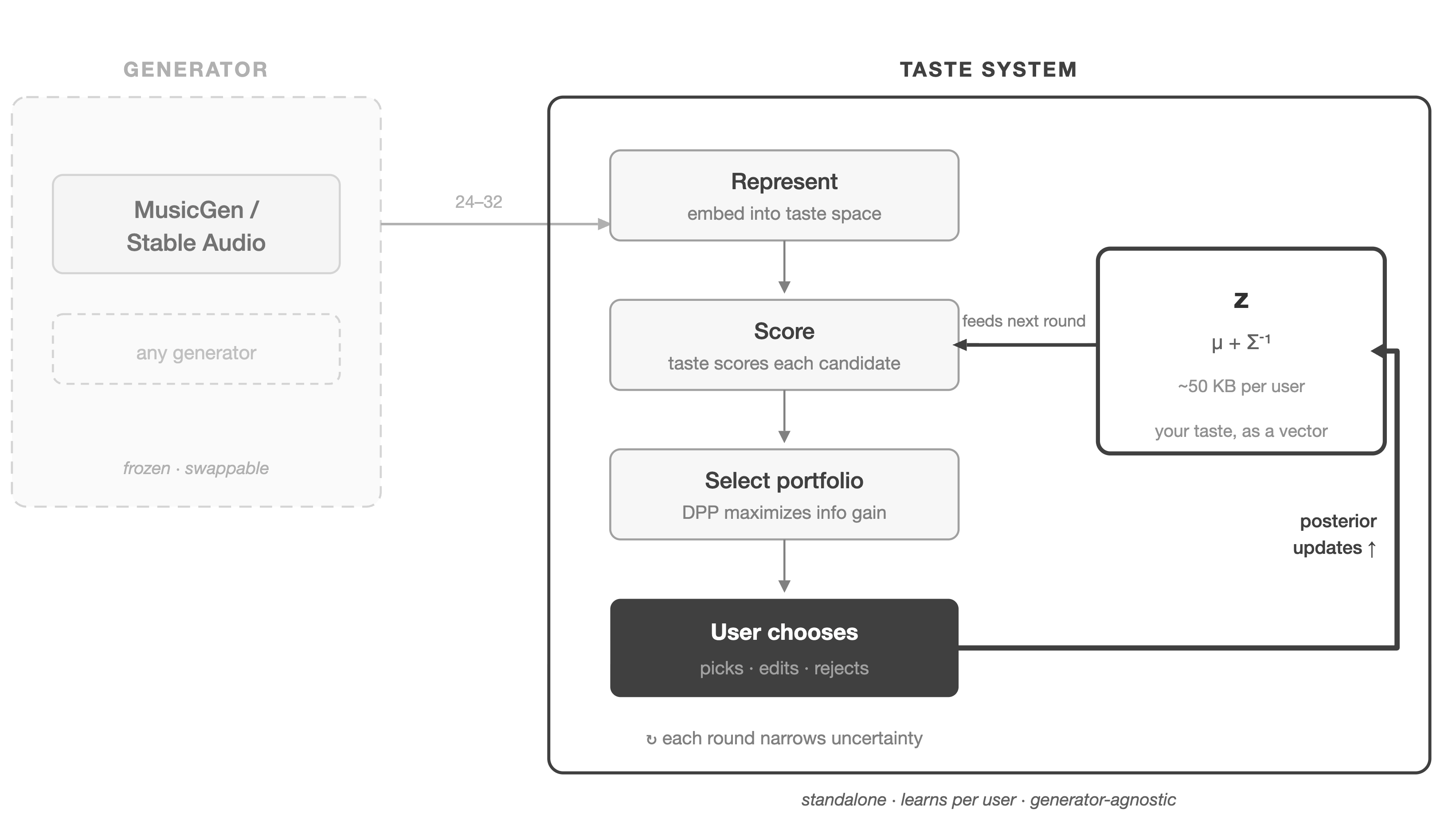
Here is the full pipeline, specifying each component at the moment it enters.
The candidate pool. The loop starts with N=24-32 candidate clips from MusicGen (or Stable Audio Open). Diversity must be engineered, because the same prompt with different random seeds gives only minor stochastic variation. The pool combines three sources of variation in roughly equal proportion: different random seeds for surface-level texture diversity, systematic prompt augmentation along taste-relevant axes (appending style modifiers like “sparse arrangement,” “dense layered,” “warm analog,” “bright digital,” “dry close-miked,” “ambient reverb” to the base prompt), and guidance-scale variation (lower scales produce more surprising outputs, higher scales stay closer to the prompt). This produces genuine spread across production style, arrangement density, and tonal character.
Representation. Each candidate passes through h_φ, the representation network that maps (audio, context, prompt) into the taste space ℝ^d where d=64. Why 64: large enough to capture the main axes of variation in CLAP’s embedding space after projection, small enough that the precision matrix Σ^{-1} remains well-conditioned in the early rounds when observations are sparse. A frozen CLAP audio encoder produces a 512-dimensional embedding e_audio. CLAP’s text encoder produces e_text from the prompt. Context c (a categorical tag like “focus” or “social,” or a free-text description) is encoded via a learned embedding or the same text encoder, producing e_context. These three vectors are concatenated into a 1536-dimensional input and passed through a two-layer MLP (1536 → 256 → d, ReLU activation). The MLP is the only learned component. The encoders stay frozen, keeping the system trainable on small per-user datasets.
A caveat: CLAP was trained on general audio, not on the production-level distinctions that matter for taste (reverb character, stereo width, compression style). The frozen encoder may collapse perceptually distinct candidates into nearby embeddings. The h_φ MLP can partially compensate, but this is the component most likely to need replacement as better music-specific encoders appear.
Each candidate’s utility is the bilinear form:
u(x) = z⊤ h_φ(x, c, y)
The taste vector z defines a direction in feature space (up to a scale set by τ and the prior), and utility is the inner product with each candidate’s representation. The prior is z ~ N(0, λ^{-1}I), with λ chosen to keep utility magnitudes O(1) relative to τ. We fix τ globally and regularize ‖z‖ through the prior, avoiding the degeneracy between choice temperature and taste magnitude. Context shifts are handled by the representation without separate per-context taste vectors.
Portfolio selection. From N encoded candidates, the system selects K=6-8 to present. The selection maximizes expected information gain about z:
I(z; choice | {x_1,…,x_K}) = H[choice | {x_1,…,x_K}] − E_z[H[choice | z, {x_1,…,x_K}]]
Exact MI maximization over subsets is combinatorial. We approximate it with a quality-weighted DPP with kernel K_ij = q_i · h_φ(x_i)⊤h_φ(x_j) · q_j, where q_i = exp(μ_t⊤h_φ(x_i)). The DPP selects subsets spanning the feature space while biasing toward high-utility regions. Exact sampling from a 32×32 kernel is cheap enough for interactive use. Among the DPP-selected candidates, the system prioritizes those with high posterior utility variance Var_z[u(x)] = h_φ(x)⊤ Σ_t h_φ(x), the points where the system is most uncertain. One or two slots are reserved for high expected utility μ_t⊤h_φ(x), so the user sees convergence alongside exploration. Early rounds (large tr(Σ_t)) favor diversity. Later rounds shift toward peak seeking. A simple schedule allocates floor(K · min(1, tr(Σ_t)/tr(Σ_0))) slots to exploration. This is a heuristic proxy for uncertainty mass, and any monotone function of posterior entropy works similarly.
The DPP kernel assumes that inner products in h_φ-space correspond to perceptual similarity. If the representation has blind spots (it will, see the CLAP caveat above), the DPP can select candidates that look diverse in the embedding but sound similar to the user. Monitoring for user-perceived redundancy in the portfolio and feeding it back as a signal is an open design problem.
A round-1 portfolio for the prompt “ambient piano” might include: a sparse reverb-heavy take, a dry close-miked version, a dense layered arrangement, a minimal two-note motif, a warm analog-processed clip, and one with prominent sub-bass. The user’s pick from this spread produces a large gradient because the candidates are far apart in h_φ-space.
The user responds. The user picks one candidate, optionally edits or explains their choice, or rejects all. The choice model is a multinomial logit, which uses the full K-way choice set in the likelihood rather than reducing to pairwise comparisons:
P(pick x_i | z, {x_1,…,x_K}, c, y) = exp(u(x_i) / τ) / Σ_j exp(u(x_j) / τ)
The temperature τ controls choice sharpness and can be inferred per event from behavioral signals like response time and deliberation patterns. Fast decisive picks imply low τ, reluctant picks imply high τ.
How the posterior updates. We maintain a Gaussian approximation to the posterior over z and update it online using the logit likelihood’s gradient and curvature. Let p_j = exp(u(x_j)/τ) / Σ_k exp(u(x_k)/τ) be the predicted choice probabilities and h_j = h_φ(x_j) the candidate representations. The gradient and Hessian of the softmax log-likelihood have closed forms:
∇_z log P(pick x_i | z) = (1/τ)(h_i − Σ_j p_j h_j)
∇²_z log P(pick x_i | z) = −(1/τ²)(Σ_j p_j h_j h_j⊤ − (Σ_j p_j h_j)(Σ_j p_j h_j)⊤)
The gradient is the difference between the chosen candidate’s representation and the probability-weighted mean, which is the “surprise” direction. The Hessian is the negative probability-weighted covariance of representations. The posterior update:
μ_{t+1} = μ_t + Σ_t · (1/τ)(h_i − Σ_j p_j h_j)
Σ_{t+1}^{-1} = Σ_t^{-1} + (1/τ²)(Σ_j p_j h_j h_j⊤ − (Σ_j p_j h_j)(Σ_j p_j h_j)⊤)
This is a small second-order update per round at d=64 (a 64×64 precision matrix, roughly 50KB per user), with no optimization loop and no backpropagation through the generator. The Hessian enforces informational asymmetry automatically. Confident choices produce large Hessians and contract the posterior substantially. Tepid choices barely register.
One risk here is that if the presented h vectors occupy a low-rank subspace (which happens when the portfolio lacks genuine diversity), the curvature update becomes ill-conditioned. In practice this means the portfolio selection stage is load-bearing for the update stage. A poorly diversified portfolio doesn’t just waste the user’s attention. It can corrupt the posterior.
Auxiliary signals. If the user provides richer feedback, additional pathways activate.
Edits. The user describes an edit (”less reverb”). The system regenerates from a modified prompt appending the edit instruction, using the same random seed to minimize irrelevant variation. The edit direction Δ = h_φ(x_i’) − h_φ(x_i) is a direct signal about which feature to move along. The loss L_edit = −z⊤Δ / (‖z‖ ‖Δ‖) pulls z to align with that direction. Seed-matching is critical: without it, stochastic regeneration variation drowns the edit signal. If the generator is not reliably seed-conditional, we approximate by generating multiple paired variants and averaging Δ. A single edit is worth roughly two to three rounds of pure choice because it identifies the specific axis rather than ranking whole candidates.
Rationales. A text rationale is encoded into embedding r via the text encoder. The contrastive loss L_rationale = −log [exp(sim(h_φ(x_selected), r)) / Σ_j exp(sim(h_φ(x_j), r))] shapes h_φ’s feature space, making it increasingly taste-relevant across users. The MLP accumulates these gradients and updates on a nightly batch schedule while z updates in real time.
Rejections. A full rejection inflates the posterior: Σ_{t+1} = Σ_t + σ²_reject · I, signaling the next round should explore broadly.
Cross-session persistence. Within a session, all updates target z_state. Across sessions, z_trait absorbs the session evidence via the mixing rule:
μ_trait ← (1 − α_trait) μ_trait + α_trait · μ̄_state^(session)
Σ_trait^{-1} ← (1 − β_trait) Σ_trait^{-1} + β_trait · Σ̄_state^{-1 (session)}
where α_trait ≈ 0.01-0.05 and β_trait controls how quickly trait-level certainty grows. z_trait is stored per user as a (μ, Σ^{-1}) pair. At the start of each new session, z_state initializes from z_trait and adapts from there.
Latency. While the user evaluates the current portfolio, the system pre-generates the next candidate pool. After the user responds, the posterior updates in microseconds, portfolio selection re-runs over the pre-generated pool with the new μ and Σ, and the next round appears with near-zero perceived wait time.
The loop in action. In round 1, maximal Σ_0 means the DPP dominates and the portfolio spans the style space. A single choice from far-apart candidates produces a large Hessian, contracting the posterior substantially. By rounds 3-5, the portfolio clusters near the estimated peak with perturbations along the most uncertain dimensions. Edits accelerate convergence on specific axes. If the user contradicts their established pattern, z_state absorbs the shift while z_trait holds. The next portfolio hedges with candidates tracking both directions. Once the primary dimensions of Σ_t are small, exploration reallocates to the orthogonal subspace, surfacing candidates the user hasn’t explored but the representation predicts they might like. This is proactive discovery, emerging from calibrated uncertainty interacting with structured representations.
3. What the System Implies
Generation is commoditizing. The taste layer is not. For mainstream prompts, generation quality is converging across MusicGen, Stable Audio, Suno, and Udio. The taste loop sits on top of any generator and is the part users actually feel. As generation becomes infrastructure, the taste layer becomes the product surface.
Taste data compounds in a way consumption data cannot. Recommendation systems learn from what you consumed from a fixed catalog. The taste loop produces counterfactual preference data: what you chose among things that didn’t exist before the system generated them. This reveals preferences in regions no catalog contains, and it feeds a flywheel: more users improve h_φ’s representation, which accelerates taste inference for new users. The taste layer is also separable from the generator, so a user’s z_trait could travel across tools and modalities.
Taste-axis design is where the domain expertise lives. What are the right prompt-augmentation axes for music versus images? Which perceptual dimensions separate human preferences, and how should they map to ℝ^d? How do you design cold-start onboarding that maximizes information gain? These questions require domain expertise fused with representation-learning fluency. This work gets more important as generators improve, because richer output spaces require more sophisticated navigation.
The failure mode that matters most is silent drift. A taste model that mislearns preferences degrades every subsequent round. z_trait drifting wrong poisons the portfolio, which produces worse choices, which reinforces the drift. The system needs calibration monitoring, drift detection, and graceful recovery designed in from the start.
4. Open Problems and Where to Start
Convergence speed. How many rounds until z outperforms random portfolios? Hypothesis: 3-5 for music (d=64, K=8), 5-10 for images. Measurable by held-out choice prediction as a function of round number.
Exploration budget. The explore-exploit schedule above is a heuristic. The Bayesian optimization literature on cumulative regret provides theoretical tools, but the empirical question in creative settings is unstudied.
Signal sparsity. Most users will only click. What is the degradation curve without edits or rationales? Measurable by ablation.
Taste drift. How should z_trait update across sessions separated by weeks? A changepoint detection layer monitoring KL divergence between z_state and z_trait, triggering faster mixing when divergence is high, may outperform simple decay.
h_φ cold start. How many users must the system see before h_φ’s feature space aligns with taste-relevant axes?
The experiment I’d run first is music generation with MusicGen or Stable Audio Open, 30-50 participants across 5-8 sessions, comparing random portfolios, choice-only learning, and full multi-signal learning against scalar RLHF and collaborative filtering baselines. Key metrics are convergence speed, held-out taste prediction (top-1/top-3 on unseen sets), and diversity among approved outputs.
Three problems worth a paper each:
Representation learning. Frozen CLAP plus linear projection as baseline versus fine-tuned versus from-scratch, measured by per-round prediction accuracy. Hypothesis: fine-tuned converges faster, with the gap largest in rounds 1-3.
Scaling laws. How does convergence scale with d, K, and population diversity? Information-theoretic arguments suggest O(d / log K) rounds in the best case. Empirical measurement versus this bound connects taste inference to rate-distortion theory.
Cross-modal transfer. Does z learned from music predict image preferences? Same users across MusicGen and Stable Diffusion (evaluated against Pick-a-Pic or HPD v2). Canonical correlation analysis between the two z vectors.
For builders. MusicGen for generation, frozen CLAP plus two-layer MLP for h_φ, softmax with per-event τ, online Gaussian updates with closed-form Hessians, DPP portfolio selection from 24-32 candidates via prompt augmentation and seed/guidance variation. Store z_trait as (μ, Σ^{-1}) per user. Pre-generate the next pool while the user evaluates the current round. The first version needs to show one thing, that taste-conditioned portfolios converge faster than random.
If I were starting this tomorrow, I would build the simplest version that closes the loop. MusicGen, frozen CLAP, softmax choices, online Gaussian updates, DPP portfolios. No edits, no rationales, no cross-session persistence. One question. Does a taste-conditioned portfolio converge faster than a random one? If it does, everything else in this post is engineering. If it doesn’t, the representation is wrong and nothing else matters.
This matters beyond music. Image generators, video generators, and code generators are all converging on the same problem. Output quality is improving faster than anyone’s ability to say what they actually want. The generation side has billions in funding and thousands of researchers. The taste side has almost nobody. That asymmetry won’t last, because the moment generation becomes commodity infrastructure, the only defensible layer is the one that knows what to generate for this person right now. Whoever builds that layer owns the interface to the entire creative stack.
References
Christiano et al. (2017). Deep Reinforcement Learning from Human Preferences. The foundational RLHF framework this work departs from.
Luce, R.D. (1959). Individual Choice Behavior: A Theoretical Analysis.
McFadden, D. (1973). Conditional Logit Analysis of Qualitative Choice Behavior.
Rafailov et al. (2023). Direct Preference Optimization: Your Language Model is Secretly a Reward Model. The dominant current approach to preference alignment. Our system addresses the per-user, online, multi-signal setting DPO does not target.
Elizalde et al. (2023). CLAP: Learning Audio Concepts from Natural Language Supervision. The audio-text encoder used as the frozen backbone for h_φ.
Kulesza & Taskar (2012). Determinantal Point Processes for Machine Learning.
Kirstain et al. (2023). Pick-a-Pic: An Open Dataset of User Preferences for Text-to-Image Generation.
Wu et al. (2023). Human Preference Score v2: A Solid Benchmark for Evaluating Human Preferences of Text-to-Image Synthesis.
Dumoulin et al. (2024). A Density Estimation Perspective on Learning from Pairwise Human Preferences.
Gao et al. (2024). PRELUDE: Aligning LLM Agents by Learning Latent Preference from User Edits. NeurIPS 2024.
Huang et al. (2025). MusicPrefs: A Large-Scale Dataset for Music Preference Prediction.
Tan et al. (2024). Democratizing Large Language Models via Personalized Parameter-Efficient Fine-tuning (One PEFT Per User).
Charakorn et al. (2026). Doc-to-LoRA: Learning to Instantly Internalize Contexts. Sakana AI.
Concepts Compilation thesis · Evaluative vs generative judgment